Thurstone Portfolio Polishing: Tail-Sensitive Black-Litterman and Beyond
We develop Thurstone portfolio
polishing: a way to take an existing allocation on the simplex—a
capitalization index, an equal-weight book, any benchmark—and re-tilt it
under a view on dependence rather than returns. Reading the
weights as the winning probabilities of a race among assets (a
Thurstonian model of choice), we back out the latent abilities that
reproduce them with a fast exact inverse, then re-evaluate the
race under a richer dependence law. The marquee instance is a
tail-sensitive analogue of Black–Litterman: where
Black–Litterman tilts a benchmark by a view on expected returns through
a linear inverse of a covariance, we tilt by a view on lower-tail
co-movement through a fast exact nonlinear inverse of a
correlated race, inverting no covariance and solving no optimization.
Driven by a tail-dependent simulation the polish shades down exactly the
names that crash together beyond what their correlation can encode—a
crash-proofing overlay we verify both in a known-truth lab and on the
Dow. The construction’s organizing property is redundancy (clone)
consistency: a near-duplicate asset splits a position rather than
doubling it—the cure for the red-bus/blue-bus failure of any Luce-type
rule, and the same near-singularity that simultaneously makes the polish
robust to ill-conditioning (it samples from a correlation rather than
inverting one), low in turnover (its weights are locally Lipschitz in
the correlation), and a smooth de-duplicator of correlated holdings. The
polish is feasible on the simplex without optimization, reproduces its
benchmark by construction, admits an arbitrary performance simulation so
dependence beyond second moments can be matched, and solves an implied
mean–(convex-regularizer) program whose penalty the simulation fixes;
capitalization weighting is its degenerate, correlation-blind member. We
prove the supporting properties (feasibility, benchmark reproduction,
redundancy and tail consistency, the implied objective, and a Lipschitz
turnover bound) and implement the method in the allocation
package, built on thurstone.
1 Introduction
We develop Thurstone portfolio polishing: a way to take an existing allocation on the simplex—a capitalization index, an equal-weight book, any benchmark—and re-tilt it under a view on dependence rather than returns. The vehicle is a race among assets: each asset draws a noisy performance, and a weight is the probability that it comes out best. The abilities driving the race are backed out of the benchmark by a fast exact inverse, and the polish is what happens when those same abilities are re-raced under a richer dependence law. The race has a second reading as a Thurstonian model of choice, which we set against the passive industry’s capitalization weighting and its implicit appeal to Luce’s choice axiom. That Lucian habit is only superficially supported by the Capital Asset Pricing Model (CAPM): what the CAPM endorses is the efficiency of the whole-universe market portfolio, a non-Lucian object no investor on a restricted universe actually holds (2.1).
The reason to read allocation as a Thurstonian rather than a Lucian choice is a single property—clone consistency: cloning an option should not create value. The same axiom is named in social choice, where it is Tideman’s independence of clones (Tideman 1987). Add a second asset that behaves almost exactly like one already held, and a sensible rule should split the position across the two near-duplicates and leave the rest of the book untouched; it must not let the duplicated exposure count twice. Everything else this paper advertises—robustness without inverting a covariance, low turnover, feasibility at scale—is downstream of meeting this one axiom with a smooth order-statistic race rather than a hard clustering or an inverse. This is the portfolio form of the red-bus/blue-bus problem that unseated the logit model in discrete choice (McFadden 1974). The logit inherits that paradox from its noise: independence of irrelevant alternatives holds exactly when the race is driven by Gumbel errors (Yellott 1977), so a race under any other law escapes it by construction. A Lucian rule—capitalization weighting included—fixes the ratio of any two weights independently of the rest of the field, so inserting a near-duplicate inflates the duplicated exposure and drains weight from everything else (Propositions 1 and 5). A Thurstonian race does not: two assets that move together compete with each other, and in the limit a co-moving pair collapses to a single horse that holds their combined weight.
Covariance-based allocators are not blind to this; they reach the same de-duplication, but lurchily. Mean–variance settles the split between near- duplicates by inverting \(\Sigma\), and the direction in which two assets become identical is exactly the direction in which \(\Sigma\) loses rank; so the population answer is right while its sample estimate, dividing through a vanishing eigenvalue, swings between the twins and flips sign with the data (Markowitz 1952). The inversion-free clustering allocators (hierarchical risk parity, the Schur-complementary family) de-duplicate by grouping instead, but discretely: the split jumps as cluster membership flips. The race de-duplicates smoothly, with a closed characterization (5) and without ever forming \(\Sigma^{-1}\).
That is the organizing idea of the paper. Redundancy is near-singularity, so three properties usually treated apart turn out to be one. The race is robust to ill-conditioning because it samples from a correlation rather than inverting one (2.4); it turns over little because its weights are locally Lipschitz in the correlation and move only as far as the correlation moves, where the clustering methods re-seriate each period (2, 8); and it splits redundant exposure gracefully. The three are one behaviour—moving smoothly along the direction in which assets become collinear and a covariance inverse would explode.
One property genuinely stands apart, because it is not about conditioning at all. Unlike any covariance functional, the race admits tail dependence: driven by a tail-dependent simulation it responds to lower-tail co-movement that no second moment can encode, so a cluster that crashes together—but only in the crash—de-duplicates in the tail (7). The winner of a race is an order statistic of the joint draw, and an order statistic reads the tail copula where a covariance cannot.
Read the other way, a winning probability is a credit as much as a weight: a redundancy-aware attribution of credit among correlated contributors. The same machinery combines forecasts, where stable combinations are known to beat the least-squares-optimal one, and we report a first study (9).
These rest on properties established below: feasibility on the simplex with neither optimization nor inversion, exact reproduction of the benchmark when the reference and target laws agree, redundancy consistency and diversification monotonicity, tail consistency, an implied mean–(convex-regularizer) objective \(w = \nabla G_S(\theta)\) for any performance law \(S\), and a Lipschitz bound on turnover (Sections 6 and 7).
2 Background
2.1 Why the CAPM does not rescue naive indexing
The passive industry defends capitalization weighting by appeal to the CAPM. We grant the CAPM in full; the point is that its support for the practice is superficial. What the model endorses is the efficiency of the whole-universe market portfolio, a non-Lucian object the indexer never holds, and that endorsement does not transfer to the restricted universes where weighting decisions are made.
2.1.0.1 What the CAPM says.
Under the CAPM every investor is a mean–variance optimizer who agrees on the expected returns \(\mu\) and on the same covariance \(\Sigma\). Two-fund separation then has each investor hold the risk-free asset together with the same tangency portfolio, proportional to \(\Sigma^{-1}(\mu - r\mathbf{1})\). Since all investors hold the identical risky portfolio, market clearing forces it to equal the supply, the capitalization-weighted market, so \(\mathrm{cap} \propto \Sigma^{-1}(\mu - r\mathbf{1})\) and the market portfolio is efficient.
Capitalization weighting is optimal precisely because the covariance is shared and the universe is the whole world: it is the one portfolio on which all investors, reasoning from a single \(\Sigma\) over all assets, agree.1
2.1.0.2 Choice and efficiency.
Given these imperfections it is natural to ask whether allocation admits other, less normative models. The choice literature offers a rich menu, and in particular two accounts long viewed as rivals in the heyday of psychometric choice theory: Thurstone’s law of comparative judgment (Thurstone 1927) and the Lucian (logit) model. They part on whether the relative standing of two options may depend on the rest of the field, and that fault line is the one that matters here.
Write \(w_i(\mathcal U)\) for the weight a rule assigns to asset \(i\) within a universe \(\mathcal U\). Capitalization weighting sets \(w_i(\mathcal U) = \mathrm{cap}_i / \sum_{j\in\mathcal U}\mathrm{cap}_j\), so the ratio \(w_i(\mathcal U)/w_j(\mathcal U) = \mathrm{cap}_i/\mathrm{cap}_j\) does not depend on \(\mathcal U\). That is Luce’s choice axiom (Luce 1959), independence of irrelevant alternatives, and we call such a rule Lucian. Efficiency has no such invariance: the tangency weights on \(\mathcal U\) are \(w^{*}(\mathcal U) \propto \Sigma_{\mathcal U}^{-1}(\mu_{\mathcal U} - r\mathbf{1})\), whose ratios turn on the entire inverse covariance \(\Sigma_{\mathcal U}^{-1}\) and move when an asset enters or leaves \(\mathcal U\) (unless \(\Sigma_{\mathcal U}\) is diagonal). The CAPM makes the two objects coincide at a single universe, the whole world, where clearing fixes \(\mathrm{cap}\propto\Sigma^{-1}(\mu-r\mathbf 1)\).
Proposition 1 (Lucian weighting is inconsistent under restriction). Capitalization weighting is the Lucian rule with values \(\mathrm{cap}_i\). If returns are correlated (non-diagonal \(\Sigma\)), then generically a Lucian rule coincides with mean–variance efficiency on at most one universe in a nested family. Under the CAPM that universe is the full asset world \(U\); on any strict sub-universe \(S \subsetneq U\) the capitalization-weighted portfolio is generically inefficient, and the discrepancy is governed by the heterogeneity of the assets’ covariances with the excluded set \(U \setminus S\).
Proof. Partition the market \(U = S \cup X\) into the retained assets \(S\) and the excluded \(X = U\setminus S\), with market weights \(m = (m_S, m_X)\). CAPM equilibrium reads \(\mu - r\mathbf 1 = \gamma\,\Sigma_U\, m\) for some \(\gamma > 0\); its \(S\)-block is \(\mu_S - r\mathbf 1 = \gamma(\Sigma_{SS} m_S + \Sigma_{SX} m_X)\), so the restricted-universe tangency weights are \[\begin{equation*} q_S \;\propto\; \Sigma_{SS}^{-1}(\mu_S - r\mathbf 1) \;=\; \gamma\big(m_S + \Sigma_{SS}^{-1}\Sigma_{SX}\, m_X\big), \end{equation*}\] while restricted capitalization weighting uses \(m_S\). The two coincide iff \(\Sigma_{SS}^{-1}\Sigma_{SX}\, m_X \propto m_S\), which holds generically only at the full universe (\(X = \varnothing\)), fixing the single coincidence point. The wedge \(\Sigma_{SS}^{-1}\Sigma_{SX}\, m_X\)—the regression of the retained assets on the excluded ones—is precisely the part of each cap weight that reflects covariance with \(U\setminus S\), irrelevant to the \(S\)-frontier yet baked into the full-market weight. ◻
The CAPM’s support for the Lucian habit is therefore the single-point coincidence of 1: it endorses cap weighting on the whole-market universe alone, and is silent, indeed contrary, on the restricted universes where weighting decisions are actually made. This is the choice-theoretic form of Roll’s critique (Roll 1977): the only testable content of the CAPM is the efficiency of the true market portfolio, and no proxy on a restricted universe inherits it (Prono 2009). We do not contradict the CAPM, only decline to extend it past its premises. Fundamental indexing reaches cap weighting’s sub-optimality by a different route, price inefficiency (Hsu 2006), while shrinkage (Ledoit and Wolf 2004) and tracking-error analysis (Roll 1992) document the fragility of the inputs.
2.2 Asset allocation as a choice
If capitalization weighting is a Lucian habit rather than a principle, what is an informationally modest alternative to naive indexing? We read allocation as a choice. The market, in aggregate, selects among assets, and a portfolio weight is the probability with which an asset is chosen. Thurstone’s law of comparative judgment (Thurstone 1927) is the canonical model of such a choice: each alternative \(i\) carries a latent quality, an ability \(a_i\), and a noisy performance \(X_i = a_i + \varepsilon_i\), and the alternative with the extreme performance is chosen. The probability that \(i\) is chosen depends on the whole field and on the dependence among the performances, the property the Lucian (logit) model forbids by axiom. Two assets that move together compete with each other, not independently, and a choice model charges for that where a Lucian one cannot.
Using these choice probabilities as weights is the construction of this paper: 4 fixes the field’s abilities by calibration to a chosen benchmark, then tilts by re-running the choice under the dependence actually realised.
The tilt is informationally modest. It needs only that dependence, no return forecast, and it anchors to the benchmark, departing from the prevailing allocation only as far as the correlation warrants. Treating the market as at least weakly efficient is the prudent default; discarding that anchor to bet against the index on thin evidence is the error that undid many entrants in the M6 forecasting competition.
2.3 Thurstone’s eclipse, and the Fast Ability Transform
The Thurstonian (probit) choice model is older and strictly more general than the Lucian (logit) one, and it does not assume independence of irrelevant alternatives. It lost the applied field on a single axis, tractability. With more than two alternatives the choice probabilities are Gaussian orthant integrals with no closed form, and the inverse problem, recovering latent abilities from observed choice shares, was considered prohibitive. Logit has closed-form probabilities and a trivial inverse, and so came to dominate discrete choice, ranking, and learning-to-rank, carrying its IIA assumption with it.
Two developments lift the obstruction here. First, the forward race is cheap to simulate: the winning frequencies of \(10^4\) to \(10^5\) correlated draws cost milliseconds, and a common-seed construction (7) makes the simulation smooth in the dependence, so it can be re-used online without churning the weights. Second, and decisively for calibration, the Fast Ability Transform of Cotton (2021) evaluates the forward and inverse maps of the independent race in linear time on a lattice, convolving competitor densities and tracking tie multiplicity exactly, so the once-prohibitive inverse from target weights to abilities is now \(O(n)\) and Monte-Carlo-free. A theoretical curiosity becomes a practical allocator.
The transform is the hinge of everything that follows. We develop several uses of the apparatus, with different benchmarks to anchor to, different reference correlations, and target simulations carrying whatever dependence one wishes to match, but each routes through this one calibration map. None is practical without a fast, exact inverse from weights to abilities; with it, the rest is sampling.
2.4 Avoiding matrix inversion
The operational fragility of mean–variance optimization is the inversion of an estimated covariance (Markowitz 1952): as \(\Sigma\) nears singularity, \(\Sigma^{-1}\) and with it the weights explode. The discipline’s responses are shrinkage toward a structured target (Ledoit and Wolf 2004) and, more radically, allocators that never form \(\Sigma^{-1}\) at all (hierarchical risk parity, the Schur-complementary family, risk parity), trading point optimality for stability and scale. The Thurstone race belongs to this inversion-free family: it samples from a correlation rather than inverting one, so it stays well posed even when \(\Sigma\) is singular or rank-deficient.
Robustness to conditioning is not robustness to tails. Every method just named is a functional of the covariance, or of a correlation derived from it. A covariance is a second moment; it summarises how assets move together on average and says nothing about how they move together in the extreme. Two universes with identical covariance, hence identical minimum-variance, HRP, Schur, and risk-parity weights, can carry entirely different probabilities of a simultaneous crash. The quantity that separates them, tail dependence, is not a moment, and no re-estimation or shrinkage of \(\Sigma\) recovers it.
2.5 The tail a covariance cannot see
Concretely: how often do the Dow’s constituents fall together, and by how much? A multivariate Gaussian fit to their daily returns, pinning the means and the full covariance, reproduces a shallow joint decline well enough, but its joint tail thins far too fast. All of them closing down on the same day is only mildly underpredicted; deepen the event and the gap widens without bound. Over 2010–2024, days on which every name fell by more than two percent occurred about eighty times more often than the fitted Gaussian allows, and beyond three percent the Gaussian effectively never produces such a day, yet two did. The direction of the asymmetry is the fingerprint: the same fit underpredicts joint crashes far more than joint rallies (1).2 The Gaussian gets the average right and the joint extreme catastrophically wrong, because the lower-tail dependence \[\begin{equation} \lambda_L \;=\; \lim_{u\downarrow 0}\mathbb{P}\!\big(U_i < u \,\big|\, U_j < u\big) \label{eq:lambdaL} \end{equation}\] is zero for the Gaussian copula and substantial in markets. No shrinkage or re-estimation of \(\Sigma\) moves \(\lambda_L\) off zero; it is invisible to second moments.
| all down by \({>}q\) | all up by \({>}q\) | |||||
|---|---|---|---|---|---|---|
| 2-4(lr)5-7 \(q\) | emp. | Gaussian | ratio | emp. | Gaussian | ratio |
| \(1.0\%\) | \(0.32\%\) | \(0.080\%\) | \(4\times\) | \(0.24\%\) | \(0.111\%\) | \(2\times\) |
| \(1.5\%\) | \(0.21\%\) | \(0.012\%\) | \(18\times\) | \(0.13\%\) | \(0.018\%\) | \(7\times\) |
| \(2.0\%\) | \(0.11\%\) | \(0.0014\%\) | \(77\times\) | \(0.05\%\) | \(0.0022\%\) | \(25\times\) |
| \(3.0\%\) | \(0.05\%\) | \({\sim}0\) | \({>}10^{4}\times\) | \(0\%\) | \({\sim}0\) | — |
A choice among assets reads the joint extreme directly. The winner of a race is an order statistic of the joint draw, and the law of an order statistic is set by the tail copula, not by the covariance. Drive the Thurstonian race with a simulation that carries lower-tail dependence and the weights respond to \(\lambda_L\): assets that crash together are recognised as the near-duplicates they become in the tail, and their shares collapse to one, which no covariance-based allocator can arrange (7). With this in view we make the construction precise.
3 The Thurstonian Model of a Field
Consider a universe of \(n\) assets. Each asset has a latent ability \(a_i\in\mathbb{R}\) and a noisy performance \[\begin{equation} X_i = a_i + \varepsilon_i, \qquad \varepsilon = (\varepsilon_1,\dots,\varepsilon_n) \sim S, \label{eq:performance} \end{equation}\] where \(S\) is any centered joint law—the simulation that drives the race—and we adopt the convention that the minimum performance wins, so that a smaller ability denotes a stronger competitor. The Gaussian \(S = \mathcal{N}(0, \Sigma_\varepsilon)\) is the workhorse, and the only case in which the calibration and smoothness results below are closed-form; but the construction—and the implementation—treat \(S\) as a black-box sampler, so a copula with genuine tail dependence, a fat-tailed or skewed law, or a structured generator are equally admissible (Proposition 7 and Section 6.4). The state price (winning probability) of asset \(i\) is \[\begin{equation} p_i \;=\; \mathbb{P}\!\left( X_i = \min_{k} X_k \right). \label{eq:stateprice} \end{equation}\] When the performances are independent (\(\Sigma_\varepsilon\) diagonal) the \(p_i\) are determined by the abilities alone through the distribution of the first order statistic, and \(p\) is a smooth, monotone function of \(a\) (Cotton 2021). Two maps are then of interest: \[\begin{align} \text{forward:}\quad & a \;\longmapsto\; p, \label{eq:forward}\\ \text{inverse:}\quad & p \;\longmapsto\; a. \label{eq:inverse} \end{align}\] The inverse [eq:inverse]—the Fast Ability Transform—recovers abilities (up to an additive constant) from a target set of winning probabilities, and is the engine of the construction below.
4 Thurstone Portfolios via the Ability Tilt
We treat portfolio weights as winning probabilities and assets as competitors. The construction uses two simulations—a reference law and a target law. We first calibrate latent abilities so that the race under the reference law reproduces a target allocation \(w^{\mathrm{target}}\) (a benchmark such as capitalization weights); we then re-run the race under the target law and read off the winning probabilities as the tilted weights. In the Gaussian workhorse the two laws are two correlation matrices—a reference \(C_{\mathrm{calib}}\) and the estimated return correlation \(C_{\mathrm{tilt}}\)—and the tilt is the portfolio’s response to \(C_{\mathrm{tilt}} - C_{\mathrm{calib}}\) (4); but any pair of centered samplers may be used, with the target law in particular carrying dependence (tail dependence included) that the reference does not.
4.0.0.1 The population map.
One display organizes the whole construction. Write \(\theta = -a\), so a larger \(\theta_i\) denotes a stronger competitor, and let \[\begin{equation} G_S(\theta) = \mathbb{E}_{\eta\sim S}\Big[\max_i(\theta_i + \eta_i)\Big], \qquad W_S(\theta) = \nabla G_S(\theta) \in \Delta, \label{eq:popmap} \end{equation}\] so \(W_S(\theta)\) is the vector of winning probabilities [eq:stateprice] (the gradient identity is 1). Calibration to a benchmark \(w^{\mathrm{target}}\in\operatorname{int}\Delta\) under a reference law \(S_0\) inverts this map, \(\theta^0 = W_{S_0}^{-1}(w^{\mathrm{target}})\) up to an additive constant (2), and the ability tilt is the composition \[\begin{equation} T_{S_0\to S_1}(w^{\mathrm{target}}) \;=\; W_{S_1}\!\big(W_{S_0}^{-1}(w^{\mathrm{target}})\big). \label{eq:tiltmap} \end{equation}\] Almost everything below is a property of [eq:tiltmap]: index reproduction is \(T_{S_0\to S_0} = \mathrm{id}\) (4); the implied objective is the Fenchel dual of \(G_{S_1}\) (1); redundancy and tail consistency are properties of \(W_{S_1}\) at the fixed \(\theta^0\) (Propositions 5 and 7); and the tilt’s smoothness is that of \(W_{S_1}\) (2). The Gaussian instance, in which \(S_0, S_1\) are two correlation matrices, is [alg:tilt] below.
Proposition 2 (Calibration). For a Gaussian reference \(S_0 = \mathcal N(0, C_0)\) with \(C_0 \succ 0\), the map \(W_{C_0} : \mathbb{R}^n/\!\operatorname{span}\{\mathbf 1\} \to \operatorname{int}\Delta\) is a smooth bijection with smooth inverse; equivalently, every strictly positive benchmark \(w^{\mathrm{target}}\in\operatorname{int}\Delta\) has a unique ability vector \(\theta^0\), modulo an additive constant, with \(W_{C_0}(\theta^0) = w^{\mathrm{target}}\).
Proof. \(G_{C_0}\) is convex (1) and, for \(C_0\succ0\), \(C^\infty\) with Hessian \(\nabla^2 G_{C_0} = \nabla_\theta W_{C_0}\), the winning-probability Jacobian, which is positive definite on the tangent space \(\{v:\mathbf 1^\top v = 0\}\) and annihilates \(\mathbf 1\) (since \(G_{C_0}(\theta + c\mathbf 1) = G_{C_0}(\theta) + c\)). Hence \(G_{C_0}\) is strictly convex on the quotient \(\mathbb{R}^n/\!\operatorname{span}\{\mathbf 1\}\), so its gradient \(W_{C_0}\) is a diffeomorphism onto the relative interior of its range, which is \(\operatorname{int}\Delta\) as any coordinate can be driven to \(0\) or \(1\) by sending abilities to \(\mp\infty\). ◻
The benchmark must lie in the open simplex: a zero target weight sends its strength \(\theta_i\) to \(-\infty\) (equivalently its ability \(a_i\) to \(+\infty\)), so zero-weight assets are dropped or floored before calibration.
Algorithm 1. Ability tilt (Thurstone portfolio)
- require target weights \(w^{\mathrm{target}}\in\Delta\); reference sampler \(S_{\mathrm{calib}}\); target sampler \(S_{\mathrm{tilt}}\) (Gaussian \(\mathcal{N}(\cdot,\,C_{\mathrm{tilt}})\) by default).
- \(a \gets \operatorname{Calibrate}(w^{\mathrm{target}}, S_{\mathrm{calib}})\) ▷ abilities s.t.\ the race under \(S_{\mathrm{calib}}\) yields \(w^{\mathrm{target}}\)
- draw \(X^{(1)},\dots,X^{(M)} \sim S_{\mathrm{tilt}}(a)\) from fixed seeds ▷ Gaussian: \(X^{(m)} = a + C_{\mathrm{tilt}}^{1/2} Z^{(m)}\)
- \(w_i \gets \tfrac{1}{M}\sum_{m=1}^{M} \mathbf{1}\!\left[\, i = \arg\min_k X^{(m)}_k \,\right]\) ▷ win frequency
- return \(w\)
Two choices of the reference correlation give the practical flavours:
Diagonal (\(C_{\mathrm{calib}} = I\)). Calibration is the exact order-statistic inverse of 3 (the Fast Ability Transform), and the tilt then injects the estimated correlation. The target may be any benchmark—the variance-only diagonal portfolio, capitalization weights, or equal weight.
One-factor market (\(C_{\mathrm{calib}} = \beta\beta^\top + \mathrm{diag}(1-\beta^2)\)). The reference is a single market factor with loadings \(\beta\); calibration reproduces the benchmark given that market correlation, so the tilt’s deviation is driven by the residual (non-market) correlation in \(C_{\mathrm{tilt}}\).
In the Gaussian workhorse a scalar \(\phi \in [0,1]\) sets \(C_{\mathrm{tilt}} = (1-\phi)\,C_{\mathrm{calib}} + \phi\,\widehat{C}\), dialling the estimated correlation \(\widehat{C}\) in continuously: \(\phi = 0\) reproduces the benchmark (4) and \(\phi = 1\) uses the full estimate. The construction never inverts a covariance—it needs only a valid correlation for sampling, repaired if necessary to the nearest correlation matrix, so the target race tolerates ill-conditioned or singular estimates (a singular \(C_{\mathrm{tilt}}\) merely makes some assets effective duplicates, with tie splitting). The reference law is different: the calibration bijection (2) and the smooth sensitivity theory (2) require a positive-definite \(C_{\mathrm{calib}}\); under a singular reference one works with limits or selected subgradients. Its feasibility, fixed-point, redundancy, monotonicity, and objective properties are established in 6.
5 Computation
5.0.0.1 Calibration (deterministic).
The calibration step—the inverse map from target weights to
abilities—is computed deterministically with the lattice machinery of
the thurstone package, which builds the distribution of the
first order statistic by convolving competitor densities and tracking
conditional multiplicity for ties (Cotton 2021). For a diagonal reference
this is the exact order-statistic inverse [eq:inverse], with no Monte-Carlo error
and cost linear in \(n\). For the
one-factor reference the assets are conditionally independent given the
market factor, so the same lattice race is evaluated at a few
Gauss–Hermite nodes and integrated over the factor; the inverse is then
a damped fixed-point on this forward map. This is the only place
quadrature enters.
5.0.0.2 Tilt (Monte-Carlo).
The race under a general target law has no tractable analytic form,
so it is evaluated by sampling. The allocation package
factors the race into a draw—the sampler—and a scoring
step, the argmin win-frequency core, so the sampler is a plug-in: the
Gaussian default recolours a fixed standard-normal ensemble by \(C_{\mathrm{tilt}}^{1/2}\) (a
quasi-Monte-Carlo ensemble may be substituted to sharpen the
win-frequency level, though not the step-to-step turnover of 7); a Student-\(t\) and a low-rank factor race (for scale)
ship alongside; and any user callable obeying the fixed-seed contract
supplies an arbitrary law. Tail consistency (7)
follows by driving the race with a downside-dependent sampler—or, within
the Gaussian workhorse, a downside (lower-partial-moment) covariance.
This supersedes the earlier winningport implementation of
the tilt.
5.0.0.3 Online updates and scale.
At rebalancing the correlation estimate moves slowly, and 7 shows the weights move smoothly with it. We exploit this by holding the standard-normal seeds fixed and transporting the path ensemble to the new correlation (recolouring by the updated square root), so turnover tracks genuine correlation change rather than sampling noise. For large universes the dense correlation is never formed: a low-rank factor model \(C = BB^\top + D\) keeps both the transport and the argmin streaming and linear in \(n\), scaling to thousands of assets. The covariance estimate itself is supplied by any external online estimator, so the method interoperates with standard covariance-forecasting tooling.
6 Theoretical Properties
We collect the properties that make the ability tilt a principled allocator rather than a heuristic. Throughout, the abilities \(a\) are fixed and we view the weights as the winning-probability map \(w(C)\).
Proposition 3 (Feasibility). For every positive-definite \(C\) and every \(a\), the weights lie in the probability simplex: \(w_i \ge 0\) and \(\sum_i w_i = 1\).
Proof. Each realization contributes one unit of weight, divided evenly among the assets attaining the minimum; summing over realizations leaves \(w_i \ge 0\) with \(\sum_i w_i = 1\). (Even division, rather than a random award among the tied, is also what keeps the estimator low-variance.) ◻
Long-only and fully-invested portfolios thus come for free—no constraints, penalties, or projection onto the simplex.
Proposition 4 (Index reproduction). If the tilt correlation equals the calibration correlation, \(C_{\mathrm{tilt}} = C_{\mathrm{calib}}\), then \(w = w^{\mathrm{target}}\).
Proof. The abilities are calibrated so that the race under \(C_{\mathrm{calib}}\) reproduces the target; evaluating at \(C_{\mathrm{tilt}} = C_{\mathrm{calib}}\) returns it. ◻
The tilt is therefore a controlled perturbation of the benchmark: the deviation is driven by \(C_{\mathrm{tilt}} - C_{\mathrm{calib}}\) and bounded by the Lipschitz estimate of 2.
Proposition 5 (Redundancy consistency). Replace asset \(k\) by two perfect duplicates \(k', k''\) (equal ability, unit variance, mutual correlation \(1\), and the same correlation as \(k\) with every other asset). Then, splitting ties evenly, \[\begin{equation*} w_{k'} + w_{k''} = w_k^{\setminus}, \qquad w_{k'} = w_{k''} = \tfrac12 w_k^{\setminus}, \qquad w_j = w_j^{\setminus}\ \ (j \neq k', k''), \end{equation*}\] where \(w^{\setminus}\) is the allocation in the original field containing the single asset \(k\).
Proof. Perfectly correlated unit-variance Gaussians with equal mean are almost surely equal, \(X_{k'} = X_{k''}\) a.s., so the field minimum—and hence every other asset’s winning event—is unchanged, while the pair ties exactly when \(k\) would have won. The even split halves that shared probability. This is a boundary case: mutual correlation \(1\) makes the correlation matrix singular, so the statement is read in the positive-semidefinite limit (equivalently, by continuity as the mutual correlation \(\uparrow 1\), with exact tie-splitting at the limit). ◻
Remark 1 (Fixed abilities versus recalibration). 5 is a statement about the race at fixed abilities: the duplicate inherits asset \(k\)’s ability. The full benchmark-anchored tilt inherits exact redundancy consistency only when calibration itself commutes with duplication, which it need not. If a duplicate enters the universe and the abilities are recalibrated to the renormalised benchmark under the independent reference, the cluster’s combined weight need not return its pre-duplication value. With a two-asset benchmark \((0.8, 0.2)\), duplicating the first asset at equal capitalisation gives the renormalised benchmark \((\tfrac49, \tfrac49, \tfrac19)\); independent calibration then sets \(|\theta_A - \theta_B| \approx 1.01\), and making the two copies comonotone gives the cluster combined weight \(\Phi(|\theta_A-\theta_B|/\sqrt2) \approx 0.76\), not the original \(0.8\). The race still de-duplicates—the copies share rather than double—but exact pre/post-universe invariance requires that duplicated assets keep their calibrated ability rather than being recalibrated through a Lucian benchmark.
This is the rigorous form of the non-Lucian advantage, though it pays to be precise about whom it indicts. At the independent extreme a duplicate is a fresh draw, so the pair’s combined weight strictly exceeds \(w_k^{\setminus}\) and draws share from every other asset—the independence-of-irrelevant-alternatives (“red bus / blue bus”) paradox. The CAPM equilibrium is not the culprit: at the whole-universe portfolio the cap weights are the efficient weights \(\Sigma^{-1}(\mu - r\mathbf{1})\), which already price a duplicate correctly through the inverse covariance. The paradox appears only when capitalization weighting is applied as a Lucian rule—normalised over a restricted universe, as in practice—where it no longer re-solves for the redundancy it carries (2.1). As the duplicate’s correlation rises from \(0\) to \(1\), 2 guarantees the pair’s share moves continuously from that Lucian value to the redundancy-coherent \(w_k^{\setminus}\). 2 shows this for three equal-ability assets.
| \(\rho_{12}\) | \(w_0\) | \(w_1 + w_2\) |
|---|---|---|
| \(0.00\) | \(0.333\) | \(0.667\) |
| \(0.50\) | \(0.384\) | \(0.616\) |
| \(0.90\) | \(0.449\) | \(0.551\) |
| \(0.99\) | \(0.484\) | \(0.516\) |
| \(1.00\) | \(0.500\) | \(0.500\) |
The monotone descent in 2 is not an accident; it holds in general.
Proposition 6 (Diversification monotonicity). Let \(T\) be a subgroup of equal-ability assets, independent of the rest of the field, with common pairwise correlation \(\rho\) within \(T\). Then the subgroup’s combined weight \(\sum_{i\in T} w_i\) is non-increasing in \(\rho\), falling from its independent value at \(\rho = 0\) to a single asset’s weight at \(\rho = 1\).
Proof. Write the within-group performances in common-factor form \(X_i = a + \sqrt{\rho}\,Z + \sqrt{1-\rho}\,\varepsilon_i\) (\(i \in T\)), with \(Z, \varepsilon_i\) independent standard normals. By Slepian’s inequality (Slepian 1962), raising the off-diagonal correlations of a Gaussian vector while fixing its marginals raises \(\mathbb{P}(\min_{i\in T} X_i > t)\) for every \(t\), so \(\min_{i\in T} X_i\) is stochastically increasing in \(\rho\). Since \(T\) is independent of the remaining field, the subgroup wins exactly when its minimum falls below the (\(\rho\)-independent) minimum of the complement; that probability is therefore non-increasing in \(\rho\). At \(\rho = 0\) the group has \(|T|\) independent chances to win; at \(\rho = 1\) it collapses to one (5 is the case \(|T| = 2\), \(\rho = 1\)). ◻
This is the diversification content of the tilt: correlated clusters are progressively de-weighted as their internal correlation rises, with no explicit risk term. The claim is exactly the one the structure affords—an equal-ability subgroup, independent of the complement, with a single equicorrelation parameter raised. We do not assert monotonicity for arbitrary clusters, correlation changes that also touch the group’s dependence with the complement, or non-Gaussian laws; the Slepian argument is what buys the stated case.
6.1 Tail consistency
We fix the sign convention for this section, since the race uses minimum-performance-wins: take \(X_i\) to be a centred loss-side performance, so a larger \(X_i\) is worse and the winner is \(\min_i X_i\). Lower-tail dependence in returns (assets crashing together) is then upper-tail dependence in these losses, and “a cluster that crashes together” is one whose loss-side performances are large together.
6 de-weights a cluster by its full correlation. Yet two clusters with an identical covariance can behave oppositely in the tail: one may crash together while the other merely co-moves on average. A symmetric second moment cannot tell them apart. If instead the race is driven by the assets’ downside dependence—approximately their co-lower-partial-moments (still a second moment, so an approximation), or, exactly, a tail-dependent joint law for the performances—the de-weighting of 6 keys to genuine tail co-movement rather than to average correlation. We call this tail consistency.
Proposition 7 (Tail consistency). Let \(G\) be a subgroup of equal-ability assets, write \(M_G = \min_{i\in G} X_i\) and \(Y = \min_{j\notin G} X_j\) with \(Y\) independent of \(G\), so the subgroup’s combined weight is \(w_G = \mathbb{P}(M_G < Y)\). Then:
If a change in the subgroup’s joint law raises \(M_G\) in first-order stochastic order while fixing \(Y\), then \(w_G\) does not increase.
In the comonotone limit \(X_i = Z_G\) for all \(i\in G\), \(M_G = Z_G\), so \(w_G\) equals the winning probability of a single competitor with performance \(Z_G\), independent of \(|G|\), and exchangeability splits it equally, each member receiving \(|G|^{-1}\).
Proof. For (i), \(w_G = \mathbb{P}(M_G < Y) = \mathbb{E}[\overline F_Y(M_G)]\) with \(\overline F_Y\) the survival function of \(Y\), which is non-increasing; a first-order stochastic increase in \(M_G\) therefore cannot increase \(\mathbb{E}[\overline F_Y(M_G)]\). For (ii), comonotonicity gives \(M_G = Z_G\), so \(\{\text{winner}\in G\} = \{Z_G = \min_k X_k\}\), the winning event of a single competitor; this does not depend on \(|G|\), and exchangeability within \(G\) splits it equally. ◻
7 is the tail analogue of 6, and it makes precise what the race responds to: not the pairwise tail-dependence coefficient \(\lambda_L\), which does not order copulas, but the whole distribution of the group minimum \(M_G\), whose lower tail is fixed by the joint lower-tail copula. As that lower-tail co-movement deepens—\(M_G\) rising stochastically while the marginals, and even the full correlation, are held fixed—the subgroup’s combined weight falls from the head-count value toward the single-competitor value, so its tail-effective cardinality runs from \(|G|\) to \(1\). For one independent asset racing a symmetric cluster that limit is \(\tfrac12\) regardless of \(|G|\). Put another way, the effective number of bets is state-dependent: in calm states \(|G|\) names may be \(|G|\) partial bets, while in a crash they are one. A covariance averages across states and cannot represent that collapse; an order-statistic race can, because the winning event is itself a tail event. Whether a given parametric family (Clayton, say, at fixed margins) deepens \(M_G\) monotonically is a family-specific question; 1 shows that it does for the family used there.
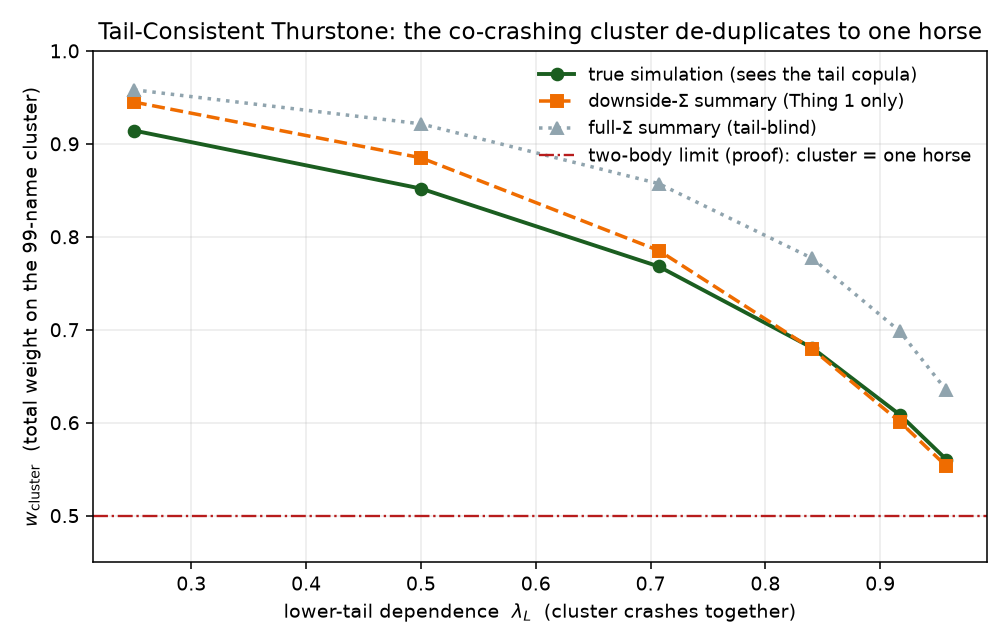
Remark 2 (Two layers of tail dependence). Full covariance is blind to the downside asymmetry (1, grey); the downside semicovariance captures the asymmetry but is still a second moment, dominated by moderate losses; the exact object is the tail copula of \(\min_{i\in G}\), which the argmin reads directly from a tail-dependent simulation and which no covariance summary represents. In the loss-side race the second-moment shadow is a close approximation (1, orange versus green), so a downside-covariance estimator suffices in practice, with the simulation path as the exact limit.
Remark 3 (Centring). The race must run on centred performances. With non-zero means the extreme order statistic tracks the lowest-drift asset and swamps the tail-dependence signal; in the tilt the abilities carry the location and the race acts on the centred residual.
6.2 The implied objective
The tilt is defined procedurally, by winning probabilities. It is natural to ask what objective, if any, it optimizes. It optimizes a recognizable one.
Specializing the population map [eq:popmap] to the Gaussian race, the expected-best potential is \[\begin{equation} G_C(\theta) = \mathbb{E}\Big[\max_i\,(\theta_i + \eta_i)\Big], \qquad \eta \sim \mathcal{N}(0, C), \label{eq:surplus} \end{equation}\] with \(\theta = -a\) (so a larger \(\theta\) denotes a stronger competitor).
Theorem 1 (Implied objective). \(G_C\) is convex and \(C^\infty\) in \(\theta\), the weights are its gradient, \(w = \nabla G_C(\theta)\), and equivalently \(w\) is the unique solution of the regularized program \[\begin{equation} w \;=\; \mathop{\mathrm{arg\,max}}_{p \in \Delta}\ \big\{\, \langle \theta, p \rangle - \Omega_C(p) \,\big\}, \label{eq:regularized} \end{equation}\] where \(\Omega_C = G_C^{*}\) is a convex regularizer (the Fenchel conjugate of \(G_C\)) supported on the simplex \(\Delta\).
Proof. \(G_C\) is an expectation of functions affine in \(\theta\), hence convex; with an almost-surely unique maximizer the envelope theorem gives \(\partial G_C/\partial\theta_i = \mathbb{P}(i = \mathop{\mathrm{arg\,max}}_k(\theta_k + \eta_k)) = w_i\), i.e. \(w = \nabla G_C\) (the Williams–Daly–Zachary identity (Williams 1977; McFadden 1981)). Equation [eq:regularized] is the Fenchel–Young duality for the convex \(G_C\) (Blondel et al. 2020); softmax and sparsemax are the special cases where \(\Omega\) is Shannon entropy or the squared Euclidean norm (Martins and Astudillo 2016). ◻
So the portfolio maximizes an ability-weighted exposure \(\langle\theta,p\rangle\) minus a convex diversification penalty \(\Omega_C\) that is determined by the correlation—a mean–(convex-risk) allocator whose feasible set is the simplex, which is why the solution is long-only and fully invested. This is the random-utility “social-surplus” / perturbed-optimizer construction (McFadden 1981; Williams 1977; Berthet et al. 2020; Papandreou and Yuille 2011). The perturbation law indexes a whole family of dependence-aware entropies—\(\Omega_S(p)\) is the cost of concentrating choice probability on \(p\) under dependence \(S\), the information cost of a rationally inattentive chooser whose logit foundation is the Gumbel case (Matějka and McKay 2015; Fosgerau et al. 2020). The choice is decisive: Gumbel noise yields \(\Omega =\) Shannon entropy and \(w =\) softmax, a correlation-blind (Lucian) allocator—the Gumbel-softmax of the machine-learning literature (Jang et al. 2017; Maddison et al. 2017); Gaussian noise with covariance \(C\) makes \(\Omega_C\) correlation-aware, which is precisely what produces the redundancy consistency of 5; a tail-dependent law makes it tail-aware (7). Spreading across independent names is rewarded; spreading across comonotone names is not—the entropy knows the dependence. Finally, since \(w = \nabla G_C(\theta)\) is the gradient of a convex potential, it is automatically smooth—\(G_C\) is a smoothing of the max in the sense of Nesterov (2005)—consistent with 2. (For general \(C\) the regularizer \(\Omega_C\) has no closed form, unlike the entropy/softmax special case, but it provably exists and is convex, which is all we use.)
6.3 Temperature and concentration
The program [eq:regularized] carries a free concentration parameter. Scaling the strengths by an inverse temperature \(\beta > 0\), \[\begin{equation} w^{\beta} = \nabla G_C(\beta\theta) = \mathop{\mathrm{arg\,max}}_{p\in\Delta}\Big\{\langle\theta, p\rangle - \tfrac{1}{\beta}\,\Omega_C(p)\Big\}, \label{eq:temperature} \end{equation}\] reweights the diversification penalty: \(\beta = 1\) is the calibrated tilt, larger \(\beta\) down-weights \(\Omega_C\) and concentrates, smaller \(\beta\) enforces it and diversifies.
Proposition 8 (Concentration with redundancy preserved). For every \(\beta > 0\) the map \(w^{\beta} = \nabla G_C(\beta\theta)\) is a simplex allocation, and
it preserves redundancy and tail consistency: equal-strength comonotone duplicates split evenly at every \(\beta\) (Propositions 5 and 7);
a strictly sub-maximal competitor (\(\theta_i < \max_j\theta_j\)) has \(w^{\beta}_i \to 0\) as \(\beta\to\infty\), the race tending to a hard \(\mathop{\mathrm{arg\,max}}\) on strength;
as \(\beta\to 0\), \(w^{\beta}\to\nabla G_C(0)\), the winning probabilities of the dependence law alone, the strengths washed out.
Proof. Scaling all strengths by \(\beta\) leaves equal strengths equal and comonotone performances comonotone, so the tie arguments of Propositions 5 and 7 are untouched, giving (i). For (ii), with \(j^\star = \mathop{\mathrm{arg\,max}}_j \theta_j\), \(w^{\beta}_i \le \mathbb{P}\big(\eta_i - \eta_{j^\star} > \beta(\theta_{j^\star} - \theta_i)\big) \to 0\) since \(\theta_{j^\star} - \theta_i > 0\). For (iii), \(G_C\) is \(C^1\), so \(\nabla G_C(\beta\theta) \to \nabla G_C(0)\) as \(\beta\to 0\). ◻
Temperature is the knob for the construction’s one residual cost. When a cluster de-duplicates, the freed weight is shared with the rest of the field, including weak competitors; by 8(ii) that leak to sub-maximal names falls to zero as \(\beta\) grows, while the even split among the duplicates is left intact by (i). The price is smoothness: as \(\beta\to\infty\) the map approaches a hard \(\mathop{\mathrm{arg\,max}}\) and the Lipschitz bound of 2 degrades, so \(\beta\) trades concentration against turnover. The calibrated \(\beta = 1\) sits at the smooth, benchmark-reproducing end.
6.4 Any simulation, and the implied penalty
Nothing in 1 uses Gaussianity. For any centred performance law \(S\) set \(G_S(\theta) = \mathbb{E}_{\eta\sim S}[\max_i(\theta_i + \eta_i)]\). This is convex in \(\theta\) for any \(S\), so the tie-split winning vector is a selected subgradient, \(w \in \partial G_S(\theta) = \mathop{\mathrm{arg\,max}}_{p\in\Delta}\{\langle\theta, p\rangle - \Omega_S(p)\}\) with \(\Omega_S = G_S^{*}\) convex on the simplex; when \(S\) is full-rank continuous this subgradient is the unique gradient \(w = \nabla G_S(\theta)\). The weights always solve a mean–(convex regularizer) program; the simulation enters only through the penalty \(\Omega_S\), which carries its full dependence, tails included.
The regularity of the gradient identity depends on the law, and three regimes are worth separating. (i) A full-rank continuous \(S\) makes \(G_S\) differentiable with an almost-surely unique maximizer, so \(w = \nabla G_S(\theta)\) and the program has a unique solution. (ii) A singular or tie-prone \(S\) (atoms, deterministic ties, duplicated coordinates) leaves \(G_S\) convex but possibly non-differentiable; the tie-split weights are then a selected subgradient \(w\in\partial G_S(\theta)\), and uniqueness or smoothness may fail—this is the regime of the exact duplicate in 5. (iii) A finite Monte-Carlo \(S\) gives a piecewise-linear empirical \(G_{S,M}\) whose weights are step functions of the parameters. The redundancy and tail results hold throughout, being statements about \(\partial G_S\); differentiability and the unique optimizer belong to regime (i).
This is the sense in which the portfolio is optimal for an arbitrary simulation. It does not claim \(\Omega_S\) is a named risk measure: only the Gumbel (Shannon entropy, softmax) and Gaussian (correlation-aware \(\Omega_C\)) cases are closed-form, and in general \(\Omega_S\) is implicit. Tail consistency (7) is precisely the statement that \(\Omega_S\) charges for tail co-movement when \(S\) carries it.
As the social-surplus conjugate, \(\Omega_S\) is a generalized entropy: it rewards spreading across independent options but counts only the dependence-effective number of bets, so it will not reward spreading across comonotone names (Propositions 5 and 7). Locally it is quadratic, its Hessian the inverse of the winning-probability Jacobian on the simplex tangent space (6.5), hence a Mahalanobis penalty in the choice geometry. It is not a coherent risk measure (neither variance nor CVaR), but the canonical Fenchel–Young regularizer of the perturbed argmax (Berthet et al. 2020).
6.5 Markowitz, reverse optimization, and the Thurstone inverse
The implied objective of 1 is best read as a reverse-optimization analogue of Markowitz. The comparison separates three roles that are easily conflated: the benchmark, the return or ability vector that rationalises it, and the risk or diversification geometry used to perturb it.
6.5.0.1 The Markowitz inverse.
The long-only mean–variance problem \(w^M = \mathop{\mathrm{arg\,max}}_{p\in\Delta}\{\mu^\top p - \tfrac{\gamma}{2}p^\top\Sigma p\}\) has first-order condition \(\mu - \gamma\Sigma w^M - \lambda\mathbf 1 = 0\), that is \(w^M = \gamma^{-1}\Sigma^{-1}(\mu - \lambda\mathbf 1)\) (ignoring binding inequalities). Expected returns are mapped to weights by the inverse covariance, and that inverse is the source of the method’s fragility: a small eigenvalue of \(\Sigma\) becomes a large eigenvalue of \(\Sigma^{-1}\), so a small return component in a near-null direction can produce a large, unstable position.
6.5.0.2 Reverse optimization.
Reverse (Black–Litterman / Grinold) optimization turns this around. If a benchmark \(w^0\) is optimal under a reference covariance \(\Sigma_0\), it implies the return vector \(\mu = \gamma\Sigma_0 w^0 + \lambda\mathbf 1\): the reverse problem applies the covariance itself, not its inverse, inferring the linear reward that would have made \(w^0\) optimal under the reference geometry. Perturbing the covariance to \(\Sigma_\phi = \Sigma_0 + \phi\,\Delta\Sigma\) while holding \(\mu\) fixed, and dropping constants and simplex-linear terms, gives the benchmark-centered program \[w^M_\phi = \mathop{\mathrm{arg\,min}}_{p\in\Delta}\Big\{\tfrac{\gamma}{2}(p-w^0)^\top\Sigma_0(p-w^0) + \tfrac{\gamma\phi}{2}\,p^\top\Delta\Sigma\,p\Big\}.\] A covariance change poses no new optimization; it perturbs the benchmark. At \(\phi=0\) the solution is \(w^0\), and for small \(\phi\) it departs only as the added penalty forces.
6.5.0.3 The Thurstone analogue.
The tilt has the same structure, with the quadratic Markowitz geometry replaced by the Fenchel geometry of the race. Calibration finds \(\theta\) with \(w^0 = \nabla G_{S_0}(\theta)\), equivalently \(\theta = \nabla\Omega_{S_0}(w^0)\) on the simplex tangent space (up to the additive constant in \(\theta\))—the analogue of \(\mu = \gamma\Sigma_0 w^0 + \lambda\mathbf 1\). Holding the score \(\theta\) fixed and tilting the law to \(S_\phi\), \[w^T_\phi = \mathop{\mathrm{arg\,max}}_{p\in\Delta}\{\theta^\top p - \Omega_{S_\phi}(p)\} = \mathop{\mathrm{arg\,min}}_{p\in\Delta}\{\Omega_{S_\phi}(p) - \nabla\Omega_{S_0}(w^0)^\top p\}.\] Adding and subtracting \(\Omega_{S_0}(p)\) writes this as \[w^T_\phi = \mathop{\mathrm{arg\,min}}_{p\in\Delta}\big\{ D_{\Omega_{S_0}}(p, w^0) + [\Omega_{S_\phi}(p) - \Omega_{S_0}(p)] \big\},\] with \(D_{\Omega_{S_0}}(p,w^0) = \Omega_{S_0}(p) - \Omega_{S_0}(w^0) - \nabla\Omega_{S_0}(w^0)^\top(p-w^0)\) the Bregman divergence of the reference regularizer. For a smooth perturbation \(\Omega_{S_\phi} = \Omega_{S_0} + \phi\,\dot\Omega_{\Delta S} + O(\phi^2)\), so \[w^T_\phi \approx \mathop{\mathrm{arg\,min}}_{p\in\Delta}\big\{ D_{\Omega_{S_0}}(p, w^0) + \phi\,\dot\Omega_{\Delta S}(p) \big\},\] the exact analogue of the reverse-Markowitz perturbation under \(\tfrac{\gamma}{2}(p-w^0)^\top\Sigma_0(p-w^0) \leftrightarrow D_{\Omega_{S_0}}(p,w^0)\) and \(\tfrac{\gamma}{2}p^\top\Delta\Sigma\,p \leftrightarrow \dot\Omega_{\Delta S}(p)\). Markowitz measures displacement from the benchmark by a quadratic form in \(\Sigma_0\); the tilt measures it by the Bregman divergence of the reference race.
6.5.0.4 Tail-sensitive Black–Litterman.
Read this way the tilt is reverse optimization with the view placed on dependence rather than on returns. Calibration backs the abilities out of a benchmark—the choice analogue of Black–Litterman’s equilibrium-implied returns (Black and Litterman 1992)—and the tilt then expresses a view on how the alternatives co-move, with \(\phi\) its confidence (\(\phi = 0\) reproduces the benchmark, \(\phi = 1\) is full conviction): exactly the role of Black–Litterman’s \(\tau,\Omega\), but over a correlation or tail view in place of a return view. That is a view Black–Litterman cannot state—“these names crash together more than the benchmark assumes” is a tail-co-movement view, not an expected-return one—and the abilities are never touched, so skill (from the benchmark) and co-movement (the view) enter as orthogonal inputs. The reverse step is genuinely nonlinear here: Black–Litterman’s implied returns are a linear first-order condition (\(\mu = \gamma\Sigma_0 w^0\), no inverse), whereas the choice geometry requires the gradient inverse \((\nabla G_{S_0})^{-1}\)—which the Fast Ability Transform (Cotton 2021) supplies exactly and in linear time. Only the simple reference law is inverted; the rich correlation- or tail-dependent target enters by forward sampling, so the prohibitive inverse of the dependent race is never formed. The closest existing device is Meucci’s entropy pooling (Meucci 2008), which tilts a scenario distribution to satisfy flexible views (tails included) and then re-optimizes; the difference is operational—the race tilts the weight vector directly on the simplex, smoothly and without a second optimization.
6.5.0.5 The displaced inverse.
Locally the two are closer still. For \(p = w^0 + \delta\), \(D_{\Omega_{S_0}}(w^0+\delta, w^0) = \tfrac12\delta^\top H_0\delta + O(\|\delta\|^3)\) with \(H_0 = \nabla^2\Omega_{S_0}(w^0)\). Convex duality gives \(H_0 = [\nabla^2 G_{S_0}(\theta)]^{-1} = [\nabla_\theta w(\theta)]^{-1}\), the inverse of the winning-probability Jacobian—here and below taken on the simplex tangent space \(\{v:\mathbf 1^\top v=0\}\), where it is positive definite, the constant direction \(\mathbf 1\) being its kernel (a Moore–Penrose inverse modulo \(\mathbf 1\)). The local penalty is \(\tfrac12\delta^\top[\nabla_\theta w(\theta)]^{-1}\delta\): a Markowitz-like quadratic with the inverse choice-sensitivity in place of \(\Sigma\). The Markowitz inverse is not replicated but displaced, from return space to choice space—\(\Sigma^{-1}\) maps returns to weights, whereas \([\nabla_\theta w(\theta)]^{-1}\) maps weight displacements to ability costs. The Fast Ability Transform is the global form of this inverse, from desired winning probabilities to abilities under the reference race. The construction is therefore inversion-free in the asset covariance—it samples from the dependence law and never forms \(\Sigma^{-1}\)—yet convex duality still leaves an inverse, now a bounded, simplex-supported curvature rather than a lever on small covariance eigenmodes. Singular dependence merely means some assets are effective duplicates in the race, not that the optimizer takes explosive offsetting positions. Numerically the contrast is suggestive: in a sweep driving the reference correlation toward singularity (condition number into the hundreds) the choice-sensitivity \(\nabla_\theta w\) stayed uniformly scaled, its own condition number near one, and a Newton calibration step preconditioned by it converged in a handful of iterations. This is an empirical observation, not a theorem, and it has a known caveat: like the softmax Jacobian, \(\nabla_\theta w\) degenerates as a weight \(w_i \to 0\), so benchmarks with very small (or floored) weights can degrade the local inverse geometry near the simplex boundary even when the dependence is well conditioned.
6.5.0.6 A selection identity.
For the Gaussian workhorse one identity sits behind this local geometry.
Lemma 1 (Selection identity). With \(X = \theta + \eta\), \(\eta\sim\mathcal N(0,C)\) for \(C\succ0\), and \(I = \mathop{\mathrm{arg\,max}}_k X_k\), the winning probability \(w_i(\theta) = \mathbb{P}_\theta(I=i)\) satisfies the selection form of Tweedie’s formula \[\begin{equation*} \mathbb{E}[X \mid I=i] = \theta + C\,\nabla_\theta\log w_i(\theta), \qquad \frac{\partial w_i}{\partial\theta_j} = w_i(\theta)\,\big[C^{-1}(\mathbb{E}[X\mid I=i] - \theta)\big]_j. \end{equation*}\] (For singular \(C\), read \(C^{-1}\) as a pseudoinverse and the identity in the limit.)
The score of the winning probability is the conditional displacement of the latent performance given that \(i\) won; the Jacobian \(\nabla_\theta w(\theta)\), whose inverse is the local penalty curvature, is a matrix of selection sensitivities. Tweedie’s identity, the Markowitz analogy, and the Fenchel dual all point to the same object: the local geometry of the winning-probability map.
6.5.0.7 Not a return forecast.
None of this makes the tilt a return-forecasting method. The linear term \(\theta\) is benchmark-implied ability, not expected return; against a true \(\mu\) the change in expected return, \((w^T - w^0)^\top\mu\), need not be positive. The claim is geometric: the tilt holds a benchmark anchor, infers the scores that rationalise it under a reference race, and perturbs under a dependence-aware race. The geometry is a diversification geometry induced by the perturbation law \(S\), not a risk geometry in return space; unless \(S\) is tied to an investor loss functional, \(\Omega_S\) rationalises the choice rule rather than supplying a welfare theorem. Its potential benefit is a better diversification geometry—fewer duplicated bets, less tail co-crash concentration, smoother turnover—while staying close to a return-bearing benchmark. The relation to capitalization weighting is then that of 2.1: efficiency on a restricted universe depends on the whole \(\Sigma_U^{-1}\), which renormalised cap weights ignore, and the tilt recovers part of that field-dependence without inversion, since assets redundant in the dependence law compete in the race and their combined weight falls with their effective distinctness. In one line: Markowitz is expected return minus a quadratic covariance penalty; reverse Markowitz reads the benchmark as an implied return perturbed by a covariance change; the tilt is benchmark-implied ability minus a race-induced convex penalty; and locally that penalty is Markowitz’s, with \([\nabla_\theta w(\theta)]^{-1}\) replacing \(\Sigma\).
7 Smoothness and Turnover
In the online (rebalancing) setting the correlation estimate moves slowly from one period to the next, and we want the portfolio to move slowly with it: turnover should track genuine change in the correlation, not estimation or sampling noise. We show the weight map is smooth, with a turnover bound, and that a common-seed Monte-Carlo realisation inherits it.
Fix the abilities \(a\) (calibrated once; they drift slowly) and view the weights as a function of the correlation matrix \(C\). Centring performances by \(a\), asset \(i\) wins iff \(Y = X - a \sim \mathcal{N}(0, C)\) lands in the fixed polyhedral cone \[\begin{equation} A_i = \{\, y : y_i - y_j \le a_j - a_i \ \ \forall j \,\}, \label{eq:wincone} \end{equation}\] so the weight is \(w_i(C) = \mathbb{P}_{Y\sim\mathcal{N}(0,C)}(Y\in A_i) = \int_{A_i}\varphi_C(y)\,dy\), with \(\varphi_C\) the \(\mathcal{N}(0,C)\) density.
Theorem 2 (Smoothness). On the open cone of positive-definite correlation matrices, \(w_i(C)\) is \(C^\infty\) in \(C\) (and in \(a\)). Moreover, on any compact subset whose smallest eigenvalue is bounded below by \(\lambda > 0\), the map is Lipschitz: \[\begin{equation} \|w(C_1) - w(C_0)\|_1 \;\le\; L_\lambda \,\|C_1 - C_0\|_F, \qquad L_\lambda < \infty,\ \ L_\lambda \to \infty \text{ as } \lambda \downarrow 0. \label{eq:lip} \end{equation}\]
Proof. The region \(A_i\) in [eq:wincone] is independent of \(C\). On the positive-definite cone \(\det C\) and \(C^{-1}\) are real-analytic, so \((C, y) \mapsto \varphi_C(y)\) is \(C^\infty\) in \(C\); its \(C\)-derivatives are polynomials in \(y\) times \(\varphi_C(y)\), which are integrable and locally dominated uniformly on compact sets. Differentiation under the integral sign then gives \(w_i \in C^\infty\). For the gradient, Price’s theorem (Price 1958)—the Gaussian identity \(\partial \varphi_C/\partial C_{jk} = \partial^2 \varphi_C/\partial y_j\,\partial y_k\) for \(j \neq k\)—followed by the divergence theorem over the cone \(A_i\) rewrites \(\partial w_i/\partial C_{jk}\) as an integral of \(\varphi_C\) over the boundary faces of \(A_i\) (the pairwise-tie hyperplanes), which is finite. The gradient is therefore bounded; since the conditioning of \(C\) controls the tie-boundary density, the bound deteriorates as \(\lambda\downarrow0\), giving [eq:lip]. (We do not claim the exact power of \(1/\lambda\); the square-root recolouring below suggests the milder \(1/\sqrt\lambda\), and the qualitative degradation near singularity is what matters.) ◻
The Lipschitz constant degrades as \(C\) approaches singularity (\(\lambda \to 0\))—the expected caveat that near-degenerate correlation makes ties, and hence weights, sensitive. This motivates keeping \(C\) well-conditioned and regenerating the path ensemble when its effective sample size collapses.
7.0.0.1 Finite paths.
2 is a statement about the population map \(w(C)\). The realized common-seed estimator \(\widehat w_M(C)\) is piecewise constant in \(C\)—it jumps when a simulated path crosses a tie boundary—so it is not literally Lipschitz. With common random numbers, \(\widehat w_M(C+\Delta C) - \widehat w_M(C)\) estimates the population difference \(w(C+\Delta C) - w(C)\) with no independent-resampling floor: its bias is zero given the shared transport, and its variability comes from paths crossing decision boundaries. Under a bounded tie-boundary density the expected number of crossing paths is \(O(M\|\Delta C\|_F)\) and each moves the weight by \(O(1/M)\), so the expected realized turnover is \(\mathbb{E}\,\|\widehat w_M(C+\Delta C) - \widehat w_M(C)\|_1 = O(\|\Delta C\|_F)\)—the population motion of [eq:lip]—with stochastic fluctuation of order \(O(\sqrt{\|\Delta C\|_F/M})\) around it. Common seeds therefore reduce the difference noise; they do not make the finite-\(M\) map Lipschitz.
7.0.0.2 Rank deficiency and conditioning.
The square root is not the inversion it replaces, and the difference is what keeps the method well posed where minimum variance is not. Inversion amplifies small eigenvalues (\(\lambda^{-1}\to\infty\)), so a rank-deficient \(\Sigma\) makes \(\Sigma^{-1}\) undefined; the root attenuates them (\(\sqrt{\lambda}\to 0\)), so a rank-\(r\) correlation merely yields draws supported on an \(r\)-dimensional subspace, a valid degenerate race whose winning frequencies still lie on the simplex. Moreover we only ever multiply by \(C^{1/2}\), never solve with it, and \(\operatorname{cond}(C^{1/2}) = \sqrt{\operatorname{cond}(C)}\), so ill-conditioning does not propagate. What degrades near degeneracy is thus not the allocation but the turnover bound: \(C^{1/2}\) is continuous through coincident eigenvalues yet only Hölder-\(\tfrac12\) there (\(\partial_\lambda\sqrt\lambda \sim \lambda^{-1/2}\)), the \(\lambda\downarrow0\) degradation of [eq:lip] (and the reason we do not pin its power tightly). The factor route of 5 removes even this: with \(C = BB^\top + \operatorname{diag}(\psi)\) the idiosyncratic floor bounds \(\lambda_{\min}\ge\min_i\psi_i\), regularizing both the root and the Lipschitz constant while never forming a dense \(C^{1/2}\).3
7.0.0.3 Common-seed transport.
We realise \(w(C)\) by Monte Carlo with a fixed set of standard-normal seeds \(Z_1, \dots, Z_M\) and the symmetric square root \(S(C) = C^{1/2}\) (itself \(C^\infty\) on the positive-definite cone): the paths are \(\widehat{Y}_m(C) = S(C)\,Z_m\) and \(\widehat{w}_i(C) = M^{-1}\sum_m \mathbf{1}[\widehat{Y}_m(C) \in A_i]\). Each indicator is piecewise constant in \(C\), flipping only when a path crosses a face of \(A_i\). A step \(\Delta C\) thus moves the realized weights by two contributions: the systematic response \(O(\|\Delta C\|)\) inherited from 2, and a sampling term from the \(O(M\,\|\Delta C\|)\) boundary crossings, which net out stochastically to \(O(\sqrt{\|\Delta C\|/M})\). Common seeds are what keep the second small: when \(\Delta C = 0\) the same seeds give the same winners and \(\Delta\widehat{w} = 0\) exactly, whereas fresh resampling carries an \(O(1/\sqrt{M})\) floor whether or not \(C\) moved. The sampling offset cancels in differences, leaving only the (smaller) crossing term, which shrinks with the path budget \(M\); this is the mechanism behind the incremental (online) update. The realized turnover is therefore not zero at finite \(M\) but is far below fresh resampling and vanishes with the path budget. (Quasi-Monte-Carlo sharpens the level of each \(\widehat{w}(C)\), but not this difference, whose noise is set by the moved decision boundary rather than by integration error.)
3 confirms both statements numerically along a \(60\)-step convex path between two random correlation matrices.
| Quantity | Value |
|---|---|
| mean \(\|\Delta C\|_1\) per step | \(0.372\) |
| mean \(\|\Delta w\|_1\), common-seed transport | \(0.0043\) |
| mean \(\|\Delta w\|_1\), fresh resampling | \(0.0145\) |
| Lipschitz ratio \(\|\Delta w\|_1 / \|\Delta C\|_1\) (max) | \(0.027\) |
| static \(\Delta C = 0\): transport | \(0\) (exact) |
| static \(\Delta C = 0\): resampling | \(0.0157\) |
8 Turnover: an empirical illustration
We claim no out-of-sample outperformance; the contribution is the construction and its properties. Two of those are visible in a plain walk-forward and matter in practice: low turnover (2) and well-posedness when names outnumber observations. For turnover we trade each estimator forward over the \(28\) Dow constituents with full 2010–2024 daily history (Yahoo Finance) from a \(252\)-day warm-up, updating online each day; turnover is the mean one-way fraction of the book traded per day, the net Sharpe charging \(10\) basis points on it.
| Method | Turnover | Sharpe | Net Sharpe |
|---|---|---|---|
| Equal weight | \(0.000\) | \(0.74\) | \(0.74\) |
| Inverse variance | \(0.005\) | \(0.78\) | \(0.76\) |
| Risk parity | \(0.004\) | \(0.78\) | \(0.76\) |
| Minimum variance | \(0.045\) | \(0.77\) | \(0.60\) |
| Hierarchical risk parity | \(0.034\) | \(0.79\) | \(0.67\) |
| Schur (\(\gamma=0.5\)) | \(0.071\) | \(0.78\) | \(0.53\) |
| Thurstone tilt | \(0.008\) | \(0.71\) | \(0.69\) |
The tilt turns over four to nine times less than the seriation-smoothed Schur and HRP and than minimum variance, in line with 2: its weights move with the correlation, not with the re-clustering or re-seriation those methods incur each step, and it sits at the low-turnover end alongside inverse variance. Gross Sharpe is comparable across methods, so the gap is not an artefact of trading little. We make no risk-adjusted-return claim.
8.0.0.1 Scale.
The second practical property is feasibility. Beyond a few hundred names (\(n > T\)) the sample covariance is rank-deficient, so the dense inverse-covariance formulas for minimum-variance and maximum-diversification (\(\Sigma^{-1}\mathbf 1\), \(\Sigma^{-1}\sigma\)) are undefined; the long-only quadratic program \(\min_{p\in\Delta} p^\top\Sigma p\) still has a solution—the simplex constraints can remove null directions—though it can be non-unique or unstable. Only the inversion-free methods stay well-behaved. The factor-form race never inverts and costs \(O(Mnk)\), staying well-posed and fitting in a few seconds to \(n = 3000\) (the Woodbury factor optimizers of 5 scale likewise, and faster).
| \(n\) | dense MinVar | Thurstone (\(k{=}5\)) | FactorMinVar | HRP |
|---|---|---|---|---|
| \(250\) | undefined | \(0.38\) | \(0.01\) | \(0.02\) |
| \(1000\) | undefined | \(0.90\) | \(0.20\) | \(0.33\) |
| \(3000\) | undefined | \(3.0\) | \(1.4\) | \(3.2\) |
The cost is that the realized turnover of 2 grows with the path budget needed for stable win frequencies at large \(n\), so the race trades compute for smoothness in a regime where dense inversion is not an option at all.
9 Forecast combination: a promising but inconclusive study
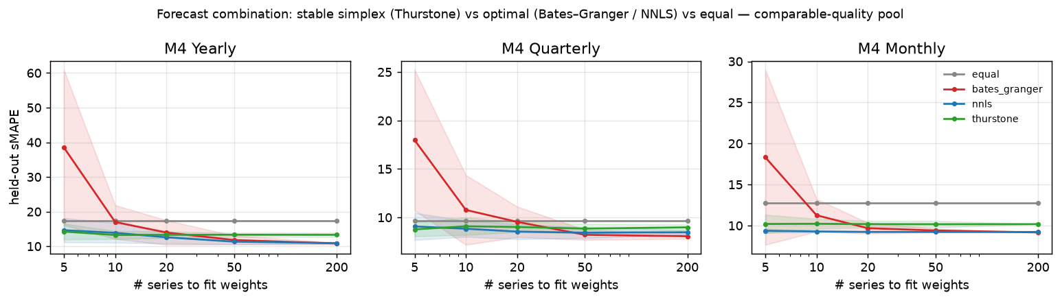
Because the tilt returns simplex weights from a dependence-adjusted regularizer without inverting anything (1), it is naturally a forecast combiner: feed the \(K\) base models’ per-period losses \(L_{k,t}\) (absolute or squared error, or an sMAPE contribution) to the race as the competitors’ performances—losses, not signed errors, so that the lowest-loss forecaster wins rather than the most negatively biased one—and read off the combination weights. Forecast combination is also where the central tension of this paper has a long empirical history—the “forecast combination puzzle” that the simple average is hard to beat with an estimated-optimal combination (Bates and Granger 1969; Timmermann 2006), precisely because the optimal weights overfit a noisily estimated error covariance.
We ran a first study on the M4 competition data (Makridakis et al. 2020), fitting the standard statistical base-forecaster pool to the Yearly, Quarterly and Monthly series, estimating combination weights on a small set of series, and evaluating held-out sMAPE while sweeping the number of fitting series—the small-sample lever the puzzle turns on (2). The result is the expected bias–variance crossover. The variance-optimal Bates–Granger combination (\(w \propto \Sigma_e^{-1}\mathbf 1\)) is wild when series are few and settles only once the error covariance is well estimated; the equal-weight average is dominated; non-negative least-squares stacking (Breiman 1996) is a strong, stable baseline. Across the swept sample sizes the ability tilt is the lowest-variance combiner, and competitive on level when forecasters are of comparable quality and the fitting data is scarce (M4 Yearly at five to ten series, Quarterly at five). Where one method dominates the pool, concentration wins and stacking takes over—exactly what the redundancy property (5) would predict. We report this as promising but inconclusive, claiming no out-of-sample superiority: the tilt is a stable small-sample member of the combination family, not a uniformly better combiner, and the case for it as a general non-negative regression and stacking tool is a direction we mean to pursue, not a result we claim here.
10 Related Work
10.0.0.1 Choice and ranking.
The Thurstonian (probit) model (Thurstone 1927) and the Luce (Luce 1959) / Bradley–Terry (Bradley and Terry 1952) / Plackett–Luce (Plackett 1975) family are the two classical accounts of probabilistic choice, differing precisely on independence of irrelevant alternatives; our allocator is the Thurstonian side of that dichotomy applied to portfolio weights (Sections 2.2 and 2.3).
10.0.0.2 The racing inverse.
Assigning winning probabilities to multi-entrant contests and inverting them to relative abilities is treated by Harville (1973) and, in the lattice form we use, by Cotton (2021); the latter supplies the linear-time forward/inverse maps and tie handling that drive calibration.
10.0.0.3 Capitalization weighting and robust portfolios.
The CAPM (Sharpe 1964), Roll’s critique (Roll 1977) and its correlation-aware refinements (Prono 2009), fundamental indexing (Hsu 2006), covariance shrinkage (Ledoit and Wolf 2004), tracking-error analysis (Roll 1992), and the Markowitz optimization baseline (Markowitz 1952) are taken up where they bear on the argument (Sections 2.1 and 2.4).
10.0.0.4 Long-only allocation as regularized regression.
Long-only mean–variance is a non-negative regression: the tangency weights are the coefficients of regressing a constant on excess returns (Britten-Jones 1999), and the no-short constraint itself acts like covariance shrinkage (Jagannathan and Ma 2003). The stable, scalable members of this family penalise that regression—\(\ell_1\) for sparse, stable portfolios (Brodie et al. 2009), portfolio-norm constraints (DeMiguel et al. 2009), and gross-exposure (\(\ell_1\)) constraints for vast universes (Fan et al. 2012). The ability tilt is the entropic member: it returns simplex weights under a dependence-adjusted entropy regularizer (1) rather than an \(\ell_1\)/\(\ell_2\) penalty, and obtains them without solving the constrained least-squares program. The same machinery is a general tool for stable non-negative (simplex) regression—it shares weight among collinear regressors (5), stays smooth under streaming updates (2), and is well-posed when regressors outnumber observations. Forecast combination and model stacking (Breiman 1996; Timmermann 2006), where stable combinations are known to beat the least-squares-optimal one, are the natural application; 9 reports a first, promising-but-inconclusive study on M4.
10.0.0.5 Perturbed optimizers.
The identity “weights equal the gradient of an expected maximum” is the random-utility social-surplus construction (McFadden 1981; Williams 1977) and, in machine learning, the perturbed-optimizer / differentiable-argmax framework (Berthet et al. 2020). Gumbel perturbations give the entropy-regularized softmax; our Gaussian, correlation-bearing perturbation gives the correlation-aware regularizer of 1.
11 Discussion
The ability tilt is a mechanically simple idea with useful properties: long-only and feasible without optimization, never inverting a covariance, reproducing a chosen benchmark by construction and tilting only in response to correlation, and solving an interpretable correlation-aware regularized program (1) whose weights vary smoothly enough (2) to bound turnover and license cheap online updates and gradient-based tuning.
Open questions include the choice of reference correlation \(C_{\mathrm{calib}}\) (diagonal versus market) and of \(\phi\); the treatment of estimation error in the abilities, a Thurstonian analogue of covariance shrinkage; and using \(C_{\mathrm{tilt}}\) to express an explicit correlation view rather than the sample estimate. The concentration of the allocation is governed by the temperature of 8, which trades the weight that leaks to weak names against the turnover bound of 2.
The tail-consistency result (7, 6.4) turns the fat-tailed-performances direction into a concrete programme: drive the race with an online downside covariance (lower-partial-moment) estimator, which 1 shows recovers almost all of the effect, and reserve the full tail-dependent simulation for the residual. Estimating that downside covariance robustly and online, and measuring whether the tail-aware tilt pays out of sample on drawdown and expected shortfall rather than Sharpe, is the natural next study.
One wrinkle we do not dwell on: investors have a well-established motivation to shrink the covariance (Ledoit and Wolf 2004), and an aggregate of heterogeneous shrunk estimates need not clear to a mean–variance-efficient market portfolio, so even the equilibrium claim is not airtight.↩︎
Daily log returns of the 28 Dow names with full 2010–2024 history (Yahoo Finance; average pairwise correlation \(0.42\)), against a Gaussian fit to their mean and covariance, the probabilities by \(10^{8}\) Monte-Carlo draws. The deepest rows rest on two to four days, so the precise multiples are noisy; the monotone, asymmetric divergence is not.↩︎
Rank deficiency is, if anything, favourable for the estimate: it lowers the effective dimension of the integrand, the regime in which quasi-Monte-Carlo excels. The eigenvalue (PCA) root loads variance onto the leading components, so a randomized Sobol’ sequence with its best-equidistributed coordinates assigned to the factor directions—the PCA construction familiar from quasi-Monte-Carlo pricing—integrates the race accurately with far fewer paths.↩︎